It is much easier for an institutional investor to operate in the stock and bond markets than in real estate because the information on these markets is so well-known and promoted and because the mechanics of investment are simple and routine. Real estate, on the other hand, requires far more analysis and marketplace involvement. Roulac cites a number of obstacles to real estate investment:

1. Objective information sources are lacking.
2. There is very limited usable research or comparable data.
3. Reliable price quotations available on a frequent basis do not exist.
4. Difficulty may be encountered in finding buyers and sellers.
5. Real estate transactions are cumbersome, time-consuming, and inefficient.
6. Because of the possibility of title imperfections, a title search and insurance policy usually is part of each transaction.
7. Negotiating the deal can be both difficult and frustrating.
8. The specialized legal aspects and the unique role of tax factors can add further complexity and cost. [1]

More serious, although curable, is the difficulty of comparing real estate and other investment media in equivalent terms.

Real estate investment performance is not now analyzed and presented in units of measure identical to those used with common stocks so that meaning­ful comparisons can be made by institutional investors. Neither does the traditional real estate literature conform to the general finance literature in its treatment of investment performance and market behavior. The task of upgrading our understanding of real estate investment is formidable yet necessary if investment real estate is to be accorded proper consideration by sophisticated institutional participants such as pension funds, bank trust departments, and insurance companies.

This paper will propose and describe a methodology that may be used to relate the performance of investment real estate to common stocks listed on the New York Stock Exchange. The procedure outlined has obvious limitations but, given the paucity of research on suitable methodologies, it may provide a useful first step to stimulate further study and development.

In 1968, the Bank Administration Institute sought to develop a measure of investment performance of pension funds that could be applied uniformly in order to make meaningful comparisons between the relative skills of asset managers. With BAI sponsorship an advisory committee directed by Profes­sor James Lorie published a report[2] which concluded that the appropriate way to evaluate performance was to consider both the return and the risk dimen­sions simultaneously. Consideration of the return dimension alone was shown to be inappropriate and often led to erroneous investment choices.

Considerable research on common stocks over the past decade has resulted in generally accepted methods of analysis for this class of investment. The re­cent shift of sizeable portfolios into the so-called “index” funds is indicative of the investment community’s acceptance of the latest concepts of portfolio theory which make both the return and risk dimensions explicit.

To close the gap between modem approaches to common stock analysis and traditional approaches to real estate investment analysis, we will show how the current techniques derived from common stocks can be applied to invest­ment real estate. Among the new ideas offered are:

1. A workable measure of investment returns,
2. A suitable measure of central tendency,
3. An appropriate measure of variability of returns about the measure of central tendency,
4. An index of comparison,
5. A measure of sensitivity of rates of return on a real estate asset or portfolio to the general market,
6. A measure of the risk premium on the real estate asset or portfolio, and
7. A measure of the degree of efficient diversification provided by a portfolio or asset.

Throughout the discussion that follows we will assume that the real estate held is in the form of a diversified portfolio. There are some problems asso­ciated with the analysis of highly undiversified portfolios or single assets[3] that are beyond the scope of this article.

Measure of Investment Returns

The starting point from which to compute the periodic rates of return on a portfolio or individual asset suggested in the BAI report and provided in data supplied by the Center for Research in Security Prices (CRSP), for instance, is the so-called “wealth relative.” The wealth relative is defined as the ratio of the value of a portfolio or asset at the end of a period to the value at the be­ginning of the period. For example, if a stock is purchased for $100 on Janu­ary 1 and has a market value of $105 one year later, the wealth relative for one year would be $105/$100 or 1.05.

The wealth relative minus 1.00 equals the rate of return achieved during the period, on the basis of the price at the be­ginning of the period. In this case the rate of return would be 0.05 or 5% for one year. If, in addition to a market value of $105 one year hence this stock had paid a dividend of $2, the wealth relative would be $107/$100 or 1.07, in­dicating a 7% rate of return for one year.

Unlike stocks, real estate generally does not have any readily identifiable mar­ket value. Appraisals are, at best, a crude measure of value and always are subject to differing interpretations. To overcome these obstacles we will make the simplifying assumptions that the starting value is the purchase price of the asset and that the income generated adds dollar-for-dollar to the value while money to cover operating losses decreases the value. If periodic appraisals are conducted, their effect can be incorporated into the changing value picture by altering the then current wealth relative. This refinement does not change the overall methodological approach but it does add another step.

This apparently naive measure of the value of real estate may strike some in­dustry practitioners as overly simplistic and unrealistic. Rather than dwell on a debate about the realism of the model, we will take comfort in Professor Milton Friedman’s comments:

“… the relevant question to ask about the ‘assumptions’ of a theory is not wheth­er they are descriptively ‘realistic,’ for they never are, but whether they are suffi­ciently good approximations for the purpose in hand. And this question can be answered only by seeing whether the theory works, which means whether it yields sufficiently accurate predictions. “[4]

Measure of Central Tendency

The early writings on portfolio theory by Markowitz,[5] Sharpe,[6] and others used the standard deviation of annual rates of return as the statistical measure of risk. The standard deviation of returns, while not the only possible measure of risk is, at least, a measure of that component of an investment which is of most concern to its owner.

The measure of central tendency must be appropriate to the available data if the measure of dispersion represented by the standard deviation is to have meaning. Other investigators have found that the geometric mean of wealth relatives minus 1.00 yields an appropriate measure of the mean rate of return. The geometric mean is used to avoid an upward bias which, in all but one special case, results when the simpler arithmetic mean is used for a compound time series. The geometric mean is not perfect but it is suitable for most prac­tical purposes.

The geometric mean rate of return is the nth root of the product of n wealth relatives minus 1.00. For example, if we had the four quarterly wealth rela­tives 1.03, 1.07, 0.98, and 1.01, the geometric mean quarterly rate of return for this series would be as follows:

R̄ = (WR₁ × WR₂ × WR₃ × WR₄)^¼ – 1
R̄ = (1.03 × 1.07 × 0.98 × 1.01)^¼ – 1
R̄ = (1.09085)^¼ – 1
R̄ = 1.04198 – 1
R̄ = 0.04198 or 4.198%

Instead of quarterly wealth relatives, we could have chosen monthly or annual wealth relatives. The choice is a matter of convenience, accuracy, and availability.

Measure of Variability

Just as the geometric mean presents a measure of central tendency. on a logarithmic scale, the measure of variability of the rates of return must also be treated logarithmically. What concerns us is a measure of the variability of returns of a given portfolio relative to the variability of returns of a general market index or market portfolio. It is this relative, not absolute, measure that must be used for comparisons.

In terms of the hypothetical real estate portfolio discussed in the Appendix, the measure of variability or risk will be the standard deviation of the natural logarithms of the quarterly wealth relatives of the portfolio for a sufficiently long series of quarters immediately preceding the time for which the compari­son of the portfolio to the market is made.

The formula for the standard deviation thus expressed is as follows:

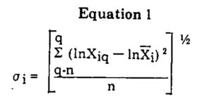
where σ_i = standard deviation. for returns of portfolio i; X_iq = wealth relative for quarter q of portfolio i;  X̄_i = geometric mean plus 1.00 of the quarterly wealth relatives of portfolio i; and n = number of quarters over which the standard deviation is measured.

We will also have use for the statistic called the variance at a later point so it should be remembered that the variance (Var_i) is merely the square of the standard deviation.

Index of Comparison

Several researchers have devised indices more or less suitable to stocks, bonds, or some combination of assets for which price movement information is rela­tively easy to obtain. Much work remains to be done to arrive at a suitable and workable index incorporating a variety of investment vehicles so that compar­isons may be made with some reliability. Lacking any better source at this time we will choose to use an index of New York Stock Exchange (NYSE) common stock returns as a reasonable proxy for an all-inclusive investment index.

Fortunately for the investment community, the Center for Research in Secu­rity Prices at the University of Chicago maintains monthly data on every common stock listed on the NYSE from 1926 to the present. The composite monthly rates of return are prepared in four ways:

1. Value weighted with reinvestment of dividends,
2. Value weighted without reinvestment of dividends,
3. Value equally weighted with reinvestment of dividends, and
4. Value equally weighted without reinvestment of dividends.

Since we will assume that our hypothetical real estate portfolio is held for the production of current income to meet pension fund obligations or the like and since real property is generally purchased in one lump, i.e., not divisible into small fungible parts, we will use the portion of the monthly rate of returns table which shows value weighted results without reinvestment of dividends.

It has been found that many commonly published indices such as the Stan­dard and Poor’s 500 Stock Index and the Dow Jones Industrial Average march together in fairly close lock-step. When one index rises, others generally do likewise. This happy result makes the selection of an index for comparison a matter of little consequence in most practical managerial applications pro­ vided that NYSE stocks are the subject of investigation. Naturally, a more comprehensive index incorporating other investment media would be helpful and desirable but, as yet, there is no such index.

Sensitivity of an Asset to the Market

The pioneering work by Markowitz in the 1950s concerned the construction of efficient portfolios of risky assets. Unfortunately, Markowitz’s solution made it necessary to know the expected return on each security, its variance and its covariance with each other security. The computational burden was clearly impossible to overcome until Sharpe suggested a simplification that would substitute the covariance of a security to the market for the covariance of each security to all other securities. For a list of 100 securities, Sharpe’s simpiifica­tion reduces the number of estimates required from 5,015 to 302. For 1,000 securities the reduction would be from 501,500 to 3,002.

Although the simplifying assumptions in Sharpe’s model tum out to have no serious detrimental effect upon the usefulness of the model when NYSE securities are investigated for conformance to predicted behavior, some as­sumptions may cause difficulty when analyzing less than efficient portfolios or less than efficient markets. Sharpe presumes that rational investors:

1. Are averse to risk,
2. Have identical time horizons,
3. Have identical expectations about the future,
4. Are immune to taxes and pay no transaction costs, and
5. Attempt to hold efficient portfolios.

By efficient portfolios we mean portfolios perfectly correlated with the market which, for a given amount of risk, yield the highest return. In theory all in­vestors would have to hold the market portfolio if perfection were attainable in all five aspects mentioned in the paragraph above.

An efficient market is one in which all known information about a security in the market is instantaneously reflected in the market price of that security. Many investigators have concluded that the NYSE is for all intents and pur­poses efficient in this sense.

The general form of Sharpe’s capital asset pricing model is:

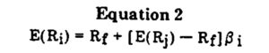
where E(R_i) = expected return on asset or portfolio i; R_f = risk-free rate; E(R_j) = expected return on the market j; and β_i = measure of the sensitivity of the return on the asset i to movements in the market.

The so-called “beta coefficient” is our measure of sensitivity. For efficient portfolios where the variability of each asset is perfectly correlated with the variability of the market, beta is equal to the ratio of the standard deviation of the portfolio return to the standard deviation of the market return, but in general, beta is given as follows:

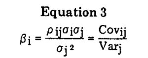
where ρ_ij =correlation coefficient between the asset or portfolio i and the mar­ket and all other terms are as defined previously.

Notice that Sharpe’s capital asset pricing model has the form of a straight line, y = a + bx. Figure 1 is a graphical representation of the model.

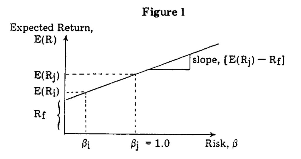
By definition, beta for the market is 1.00. Thus, it is easy to determine the expected value of a portfolio or asset return given just the risk-free rate, R_f; the expected value of the market return, E(R_j); and the beta for the portfolio or asset, β_i, For instance, if R_f= 3%. E(R_j) = 12% and β_i = 0.5, the expected return on i would be:

E(R_i) = 0.03 + (0.12-0.03) 0.5
E(R_i) = 0.03 + (0.09) 0.5
E(R_i) = 0.075 or 7.5%

Our analysis in the Appendix will show that the covariance and beta coeffi­cient for our hypothetical real estate portfolio are 0.00165 and 0.20320 re­spectively. The absolute value of the covariance has little significance for us except to note that the return on our real estate portfolio generally increases when the return on the market increases but the covariance is only slightly positive and not statistically significant. The beta coefficient does provide more useful information, namely that the real estate portfolio in our example exhibits considerably less systematic risk or volatility than the market.

The Risk Premium

The total risk or variability of an asset or portfolio is comprised of two com­ponents: nonsystematic risk and systematic risk. Nonsystematic risk can be eliminated by diversification, i.e., the inclusion of additional risky assets to make the correlation of the portfolio to the market as close to 1.00 as possible. Systematic risk, on the other hand, is that risk which remains associated. with the portfolio and cannot be eliminated through further diversification.

The theory of price in capital markets argues that since investors seek to hold efficient portfolios, the market will not pay a premium for risk which may be eliminated through diversification. The risk premium, or the amount the mar­ket will be willing to pay for an asset or portfolio above the risk-free rate, will depend entirely on the level of its undiversifiable risk. For portfolios which fall along the capital market line, the undiversifiable risk will be the total risk for naively selected efficient portfolios. Clearly superior management will be that management which can pick portfolios that in their undiversifiable or systematic risk produce a return greater than that of a naively selected effi­cient portfolio of identical risk.

We may understand the nature of the risk premium and its relationship to managerial performance by examining the results of our sample problem as shown graphically in Figure 2.

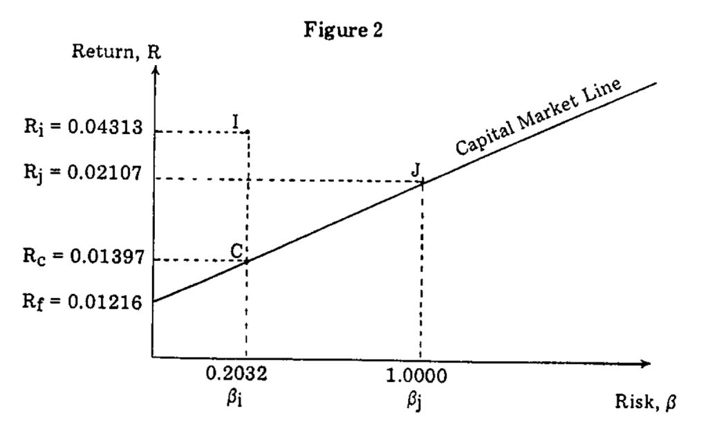
The risk-free rate, R_f, that we have supplied is the mean quarterly rate of re­turn on three-month Treasury Bills which generally serves as a good proxy.

Points I and J represent the risk-return coordinates of our hypothetical real estate portfolio and the NYSE market index respectively. Point C represents the risk-return coordinates for a naively selected efficient portfolio with the same beta coefficient as our real estate portfolio.

Clearly, our portfolio has exceeded the performance of the naively selected efficient portfolio by an amount equal to R_i – R_e. This vertical distance be­tween R_i and R_e is a measure of the portfolio manager’s ability to select a portfolio which outperforms a naively selected portfolio but it says nothing about whether the performance results from a well-diversified portfolio or from a poorly diversified portfolio.

Measure of Diversification

We have said that total risk is comprised of systematic (diversifiable) risk and nonsystematic (nondiversifiable) risk. The risk premium for a given sensitiv­ity to the market, i.e., the rate of return premium above a naively selected efficient portfolio for a given beta coefficient, is attributed entirely to the amount of nonsystematic risk. Therefore, it is useful to be able to measure the fraction of total risk attributable to the lack of diversification in the portfolio.

The proper unit of measure is derived from the correlation coefficient, ρ_ij, of the portfolio under investigation to the comprehensive general market index.

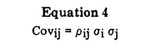
If we consider the earlier equation for the beta coefficient, we will notice that the covariance of the portfolio with the market is equal to the product of the correlation coefficient, the standard deviation of returns of the portfolio and the standard deviation of returns of the market. Symbolically, the equation is as follows:

Rearranging this formula we have the equation for the correlation coefficient:

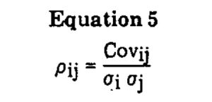
The square of the correlation coefficient ρ_ij² (or more popularly called R²) is the coefficient of determination. It measures the fraction of the total variance of the portfolio under investigation that is explained by the portfolio’s move­ment with the market. In other words, the coefficient of determination, R², is the fraction of the total risk which is systematic. One minus R² would be the fraction of the total risk which is nonsystematic and attributable to the lack of complete or efficient diversification. In the following section we will argue that specification of both the correlation coefficient (and by implication the coefficient of determination) and the beta coefficient are proper, appropriate, and sufficient descriptions of an operational investment policy.

Investment Policy

Despite the fact that investment policies of large institutional investors are generally contained in a written statement. the methods of choice among in­vestment opportunities tend to be arbitrary and the manner of control of the portfolio risk or variance is, at best, vague. Lorie and Hamilton cite three criteria commonly included in traditional investment policy statements:

1. A list of securities eligible for purchase-the so-called “buy” list.
2. A diversification requirement, usually specifying the maximum percentage of a portfolio that can be invested in the securities of a single company and the maxi­mum percentage that can be invested in a single industry.
3. A maximum percentage that can be invested in equities. [7]

No matter how detailed these criteria are, it is easy to see that the control that they might exert over the behavior of an asset manager is minimal. Within the constraints imposed by traditional investment policy statements there are a number of possible portfolios that will satisfy the stated objectives but will have widely different risk characteristics. For instance, it would be possible for an asset manager to choose to include all high beta stocks from the “buy” list into the portfolio which would result in a much riskier posture than the invest­ment policymakers intended. If we are to believe that risk aversion is a pri­mary goal of most investors, then it is incumbent that we have a good mea­sure of relative risk and an operational means of monitoring that risk.

Thus, we believe that a more precise specification of investment policy must include two measures: the beta coefficient and the correlation coefficient. By specifying a range of beta coefficients for an investment portfolio acceptable to management, we would have an explicit statement of the desired risk position relative to the market and the direction that adjustments might t.ake from time to time to adhere to a stipulated policy. For instance, if the beta coefficient were greater than desired, we would then seek to remove high beta assets from the portfolio or add lower beta assets to bring the sensitivity of the portfolio to the market back into line. Beta would help us identify the assets which could best accomplish our objectives and would offer an early warning system to alert managers to unfavorable changes.

The correlation coefficient is our measure of diversification. Above average returns which are the result of superior performance of a diversified portfolio are to be preferred by risk averse investors to above average returns from an undiversified portfolio. Also, when rating the relative skill of various asset managers and the portfolios they operate, it is important to know whether their apparent skill is achieved through undiversified investments which typically do not sustain a high level of performance or through diversified in­vestments which react less erratically to fluctuating economic conditions.

Thus, we have in the beta coefficient and the correlation coefficient a set of specifications which will enable the institutional investor 1) to define an in­vestment policy, 2) to monitor compliance with the policy, and 3) to evaluate the performance of asset managers.

To Buy or Not to Buy Real Estate

One of the most prevalent myths circulating among investment managers today is that a pension fund should not have more than 10% of its assets in­vested in real estate. It is thought that real estate is too “risky” and therefore should only be accorded a minor role in institutional portfolios.

Notice that we were able to completely specify the desired performance char­acteristics of an investment portfolio with just the beta and correlation co­efficients. Not once during the foregoing ·discussion was it necessary to men­tion the proportion of total assets to be invested in any one category of assets. Indeed, we used a hypothetical real estate portfolio for analysis but the methodology would have been identical had we chosen stocks, bonds, an­tiques, old cars, sea shells, or any other investment for which value determina­tions over time are possible.

The whole point of our discussion has been that there exists a standard ana­lytical method for investigating performance characteristics of investments. By employing a common language we can remove the myths and mysticism surrounding different investment vehicles and thereby make more rational in­vestment decisions.

To demonstrate the fallacy of such intuitive judgments as limiting a portfolio to only a given percent of a particular asset, we will use the results of our hypo­ thetical real estate portfolio and the NYSE common stock index in a com­bined portfolio. Assume for the moment that we currently have a portfolio j represented by the NYSE market portfolio but are considering the addition of some of the hypothetical real estate portfolio i. We would like to analyze the performance that might be expected of the combined portfolio assuming that past performance is a sufficiently good indicator of future performance. Initially we will consider a combined portfolio made up of 90% NYSE market portfolio shares and 10% hypothetical real estate portfolio shares.

The expected quarterly return is just the weighted average of the quarterly returns of the NYSE market portfolio and the real estate portfolio.

Where R_p = expected quarterly return on the combined portfolio; R̄_i and R̄_j= quarterly returns on the real estate portfolio i and the NYSE portfolio j; Ƶ_i = proportion of the combined portfolio invested in i; and Ƶ_j = proportion of the combined portfolio invested in j.

R_p= (0.10) (0.04313) + (0.90) (0.02107)
R_p = 0.004313 + 0.018963
R_p = 0.02328 or 2.328%

The variance of returns of a combined portfolio is not the weighted average of the respective variances except in the special case where the two assets are per­fectly correlated. The correct general form of the equation for the variance of returns for a combined portfolio of two assets is as follows:

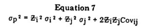
where σ_p² = variance of returns of the combined portfolio and all other terms are as previously defined. In our example, the variance would be:

σ_p² = (0.10)² (0.00218) + (0.90)² (0.00812) + 2(0.10) (0.90) (0.00165)
σ_p² = 0.00670

Two results are worthy of note. First, the expected return of the combined portfolio is greater than the return on the NYSE stock portfolio by itself (0.02328>0.02107). Second, the variance of returns of the combined portfolio is lower than the variance of returns on the NYSE stock portfolio by itself (0.00670 <0.00812).

The same pattern of results would have occurred if we had chosen to include more of the real estate portfolio relative to the stock portfolio. The following are possible outcomes for combined portfolios made up of different propor­tions of the two assets:

Proportion Invested In		Combined Results
Real Estate	Common Stocks	Rate of Return	Variance of Returns
0.10	0.90	0.02328	0.00670
0.20	0.80	0.02548	0.00581
0.30	0.70	0.02769	0.00487
0.40	0.60	0.02989	0.00406

As the proportion of real estate in the combined portfolio is increased the re­turn and variance components improve. In general, the combined variance will decrease as uncorrelated assets are combined into a new portfolio. The combined rate of return may or may not increase but the reduction in overall variance may be sufficiently attractive to sacrifice some overall return for more income stability. Intuitive judgments concerning these factors could easily have resulted in incorrect conclusions and are clearly not definable or testable.

Conclusion

Fiduciary responsibility on the part of asset managers demands a high level of expertise, analytical ability, and factually-based judgment. There can be no excuse for using outmoded methods and seat-of-the-pants judgments when techniques are available to do a better job. Neither real estate nor any other popular investment medium need be considered a case apart; the methods and language of analysis do exist and they should be applied to real estate as well as to other assets.

Several tools have been presented which can be used to organize the necssary data gathering system for any investment portfolio. We have proposed a mea­sure of wealth relatives as a starting point. The rest of the calculations are straightforward and result in two extremely important statistics: the beta co­efficient and the correlation coefficient. These two coefficients enable us to describe investment policies in a clear and unambiguous way, to monitor the performance of our portfolio over time and to make the task of evaluating different asset managers easy.

Just as participants in the stock market benefit from more information about individual stocks and the performance of the market in general, so too can real estate participants profit from more and better data presented in a stan­dardized and understandable manner. This paper has suggested the kinds of information that are needed to make real estate analysis comparable to com­mon stock analysis and therefore more acceptable and understandable to institutional participants. The task of upgrading information about real estate will not be easy, but it will be rewarding.

Appendix

---

References

1. Stephen Roulac, Modern Real Estate Investment, An Institutional Approach (The Property Press. 1976) pp. 49-50.

2. Bank Administration Institute, Measuring the Investment Performance of Pension Funds (Park Ridge, lll.: 1968).

3. Single assets cannot be considered efficient in the sense of eliminating nonsystematic (diversifiable) risk but properly diversified portfolios have reduced the nonsystematic risk to zero. 11ris point should become apparent later.

4. Milton Friedman, Essays in Positive Economics (Chicago: University of Chicago Press, 1953) p. 15.

5. Harry M. Markowitz, Portfolio Selection: Efficient Diversification of Investments (New York: John Wiley & Sons, Inc., 1959).

6. William F. Sharpe, “Capital Asset Prices: A Theory of Market Equilibrium Under Conditions of Risk,” Journal of Finance (September 1964) pp. 425-442.

7. James H. Lorie and Mary T. Hamilton, The Stock Market: Theories and Evidence (Homewood. Ill.: Richard D. Irwin, Inc., 1973) p. 264.